
1.Sycomore documentation
Version 2024
This documentation is for Sycomore starting from 2019 version.
©Lixoft
Sycomore is an application for the visual and interactive exploration of your models. It enables to keep an overview of the Monolix runs and compare them side by side.
Short overview of Sycomore
Detailed overview of Sycomore
Interface
The interface of Sycomore is separated in two main tabs displayed on these figures:
 |
 |
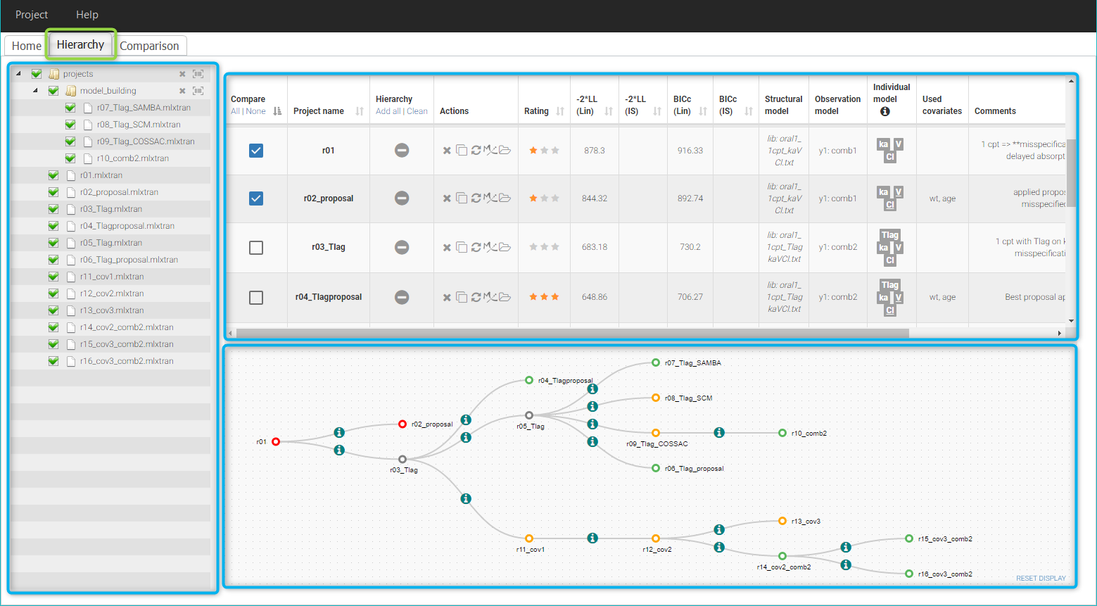
- Hierarchy tab. The hierarchy tab provides an overview of the Monolix runs. It is composed of three panels:
- Projects selection: the panel on the left allows to select Monolix projects in a list of folders chosen by the user.
- Table of projects: the panel on top shows a quick overview of selected Monolix projects as a table, with information on each project’s definition and results.
- Tree representation: the panel on the bottom provides a schematic representation of the modeling workflow as a tree of projects.
- Comparison tab. To compare the results of several runs side-by-side.
Follow the links to read detailed descriptions of each part of the interface.
File
Sycomore projects are saved as text files with the extension .syc. A sycomore project contains relative paths to the Monolix runs described in the overview.
1.1.Table of projects
The panel on top shows a table overview of the Monolix runs selected in the Selection panel, that has the following functions, detailed on this page:
- Displaying key information on each Monolix run
- Elements from the projects: project name, structural morel, error model, covariates, correlation groups, comments
- Objective function and BICc from the results
- Performing actions on each run
- Running one or several projects in Monolix
- Opening a project in Monolix or opening its result folder
- Cloning a project
- Updating the elements and results of a run
- Modifying elements of the Sycomore overview
- Including projects as nodes in the tree view
- Changes from parent nodes
- Selecting projects for side-by-side comparison
- Removing a run from the table
- Rating
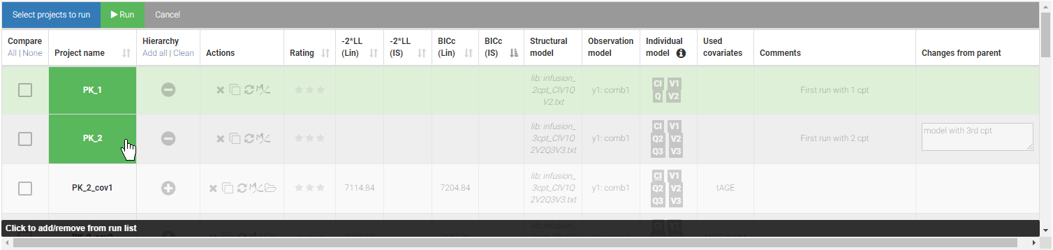
An example is shown below:
Displaying key information on each Monolix run
Elements from the projects
The name of the projects displayed in the table are the file names without the .mlxtran extension. If several projects from different folders have the same name, the name of the folders are also added to distinguish them. It is possible to sort the table rows by project name.
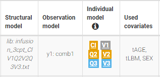
The main elements of the structural and statistical models from each Monolix projects are displayed in the columns:
- Structural model: the path to the structural model
- Observation model: the error model chosen for each observation id (const=constant, prop=proportional, comb1=combined1, comb2=combined2)
- Individual model: the names of the parameters are displayed. They are underlined if they are involved in covariate effects, in italic if they have no variability, and colored if they are part of correlation groups.
- Used covariates: covariates that are used in the statistical model.
An example if shown below, where the structural model is the file infusion_3cpt_ClV1Q2V2Q3V3.txt from the PK models library, the error model is combined1, the individual parameters Cl, V1, Q2, V2, Q3 and V3 all have random effects are all have some covariate effect, among the covariates tAGE, tLBM, SEX. There are also two correlation groups: {Cl, Q2, V2} and {Q3, V3}.
The column Comments displays all comments saved in the Monolix projects. Note that markup or mardown formatting is not applied.
Objective function and BIC from the results folders
The log-likelihood and corrected BIC are displayed in the columns:
- -2*LL (Lin): -2*log-likelihood computed by linearization,
- -2*LL (IS): -2*log-likelihood computed by importance sampling,
- BICc (Lin): corrected BIC based on the log-likelihood computed by linearization,
- BICc (IS): corrected BIC based on the log-likelihood computed by importance sampling.
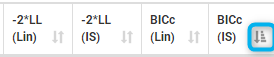
Table rows can be sorted in increasing or decreasing order according to each of these columns with the sorting icon, as seen here:
Performing actions on each run
Running one or several projects in Monolix
The table can be used to select projects in a run list that can be run together in a row. This is done by clicking on each project name, as can be seen below. A button “Run” appears, it runs the scenario defined in each project. The results are then automatically updated in the table.
Action buttons
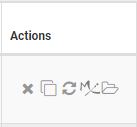
The column named Actions contains a set of buttons, seen above, to perform useful actions. Their functions are:
 Remove the project from the table. This does not remove the project from the Selection panel.
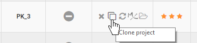
 Clone a project: this action asks for a new name, a copy of the project is saved under this name.
 Update the elements and results displayed for the project
 Open the project in Monolix
 Open the result folder of the project
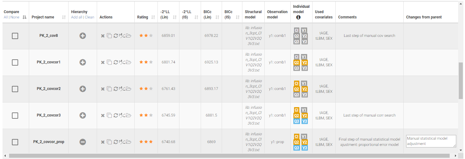
Modifying elements of the Sycomore overview
Several elements of the table can be modified and saved in the Sycomore project.
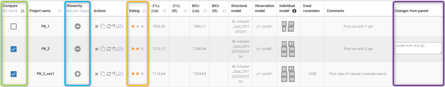
- Selecting projects for side-by-side comparison (see green mark above): this is done by checking bowes in the column named “Compare”. The selected projects are then displayed in the Comparison tab.
- Including projects as nodes in the tree view (see blue mark above): with buttons in the column named “Hierarchy”.
- Rating (see orange mark above): by clicking on the stars in the column Rating. The ratings then appear as a color code in the tree view (*: red, **: orange, ***: red).
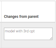
- Changes from parent nodes (see purple mark above): text fields for projects that have a parent in the tree diagram can be filled directly in the column named “Changes from parent”, or in the tree diagram.
1.2.Selection panel
The panel on the left of the Hierarchy tab allows to select Monolix projects in a list of folders chosen by the user. Selected projects appear in the Table part of the interface, and can then be added in the Tree representation and/or in the Comparison tab.
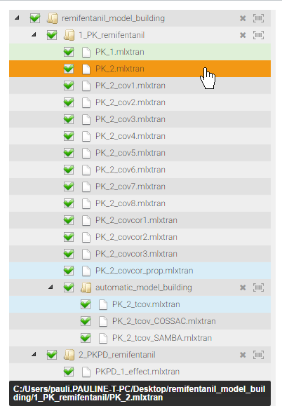
Hovering on a project in the list displays its absolute path at the bottom. It also highlights the project in orange in the Table and Tree representation in the interface. Moreover, if the project is included in the tree representation, its parent is highlighted in green and its child(ren) is(are) highlighted in blue.
Adding a project in the list
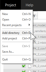
A new project can be added in the selection list by clicking on “Add project” in the Project menu, and selecting a Monolix project (.mlxtran file) in the browser.
It is also possible to click “Add directory” and select a folder in the browser. In that case all Monolix projects contained in the folder are displayed in the selection list, and are by default unselected.
If several projects appear in the list, the hierachy of folders up to the closest common root is displayed as well.
Selecting projects
Projects can be selected one-by-one, or all the projects in a folder can be selected together by selecting their folder.
The list of projects in a folder can be updated with the button “Rescan directory” as below:
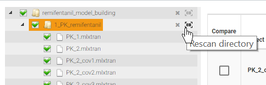
Next to the button “Rescan directory”, the cross icon permits to remove a directory from the list.
1.3.Tree view
The panel on the bottom of the Hierarchy tab provides a schematic representation of the modeling workflow as a tree of projects. This graph diagram is built by the user and contains:
- the name of the Monolix projects
- changes from the parent project
- the rating of the projects is displayed with a color code
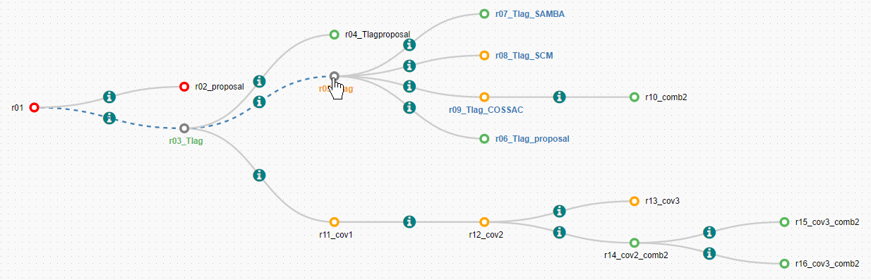
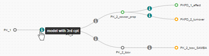
As seen on the figure above, hovering on a node of the diagram highlights its parent in green and its child(ren) in blue, on the diagram but also in the Selection panel and the Table of runs. The path to the root node is also displayed in dashed blue line.
Building the tree representation
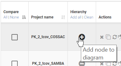
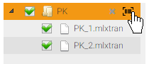
To build the tree representation of your workflow, use the buttons “Add node to diagram” (shown below) in the table of projects to add relevant projects in the tree view.
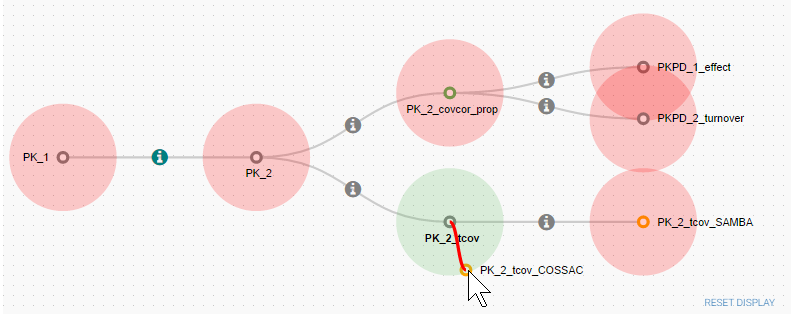
The projects are first added in the tree view as free nodes. They can be linked to a parent node via drag-and-drop. Available nodes are then highlighted in red, and the selected parent is highligted in green, as on the following figure.
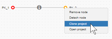
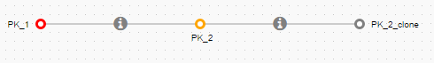
Cloning a project allows to create a copy of the Monolix project with a different name, that can then be opened in Monolix and modified. A clone is automatically added in the tree view as the child of the cloned project.
 |
➞ |
 |
Defining parent-child relationships
Changes from the parent project can be saved and displayed on the graph edges and in the table of projects.
| Two ways to define a parent-child relationship | Display on hover |
|---|---|
 |
 |
 |
Display of rating
The rating of runs set manually in the table of project is displayed with a color code on the tree view: red for one star, orange for two stars, green for three stars.
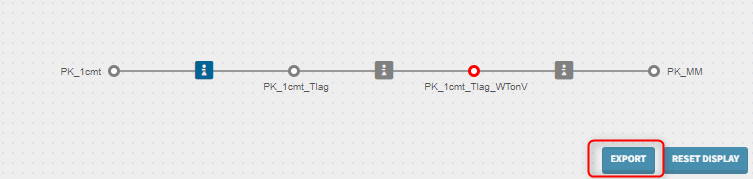
Export
Starting from the version 2024, it is now possible to export the tree as an SVG file by clicking on the export button next to the tree. The exported tree will be the same as the tree in the interface, however it will not contain the information icons.
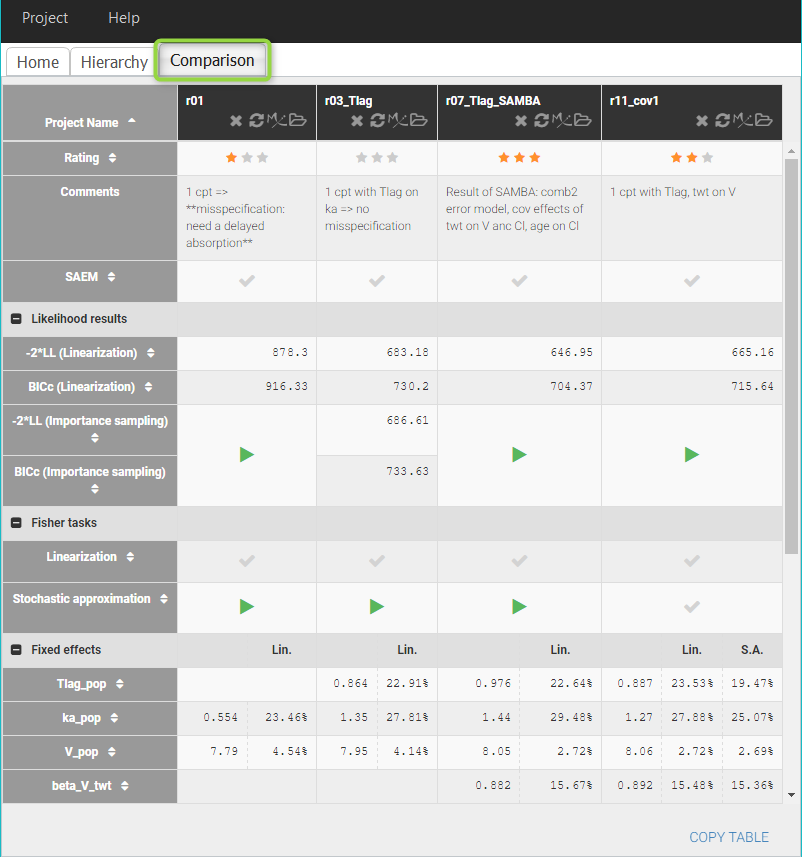
1.4.Comparison
The comparison tab allows to compare side-by-side the main results of a set of Monolix projects selected in Sycomore.
Monolix projects are selected for comparison in the Table overview of the Hiearchy tab.
The results include:
- Project information:
- Project name
- Rating: the rating given to the projects in Sycomore. They can be changed on this table or in the Hierarchy tab.
- Comments: the comments saved in each Monolix project
- SAEM: this row indicates for each project whether the population parameters have been estimated.
- Likelihood results: the values of -2*LL and BICc based on the log-likelihood computed by linearization or by importance sampling
- Fisher tasks: these rows indicate for each project whether the Fisher information matrix by linearization or by sochastic approximation has been computed.
- Fixed effects: estimates and standard errors for the fixed effects (omega parameters)
- Standard deviation: estimates and standard errors for the standard deviations of the random effects (omega parameters)
- Residual error parameters: estimates and standard errors for the parameters of the residual error model
- Figures: diagnostic plots exported as png images
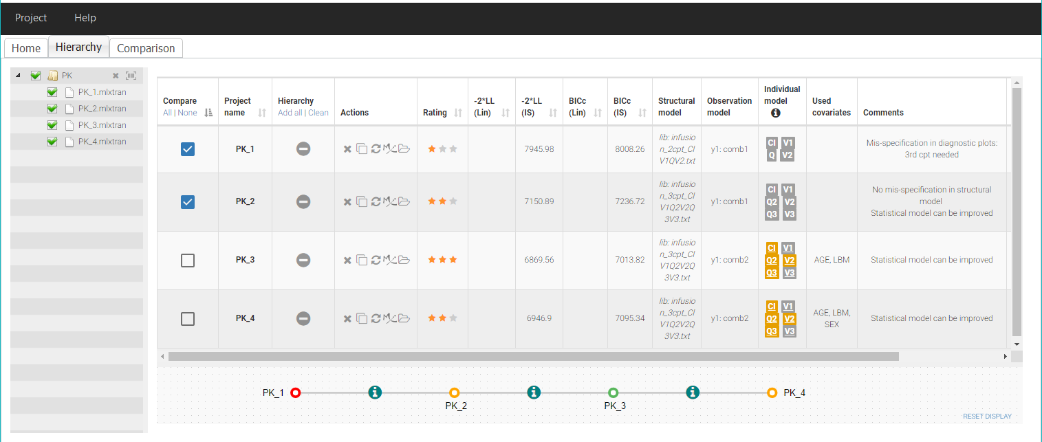
Here is an example of the table Comparison with 4 projects:
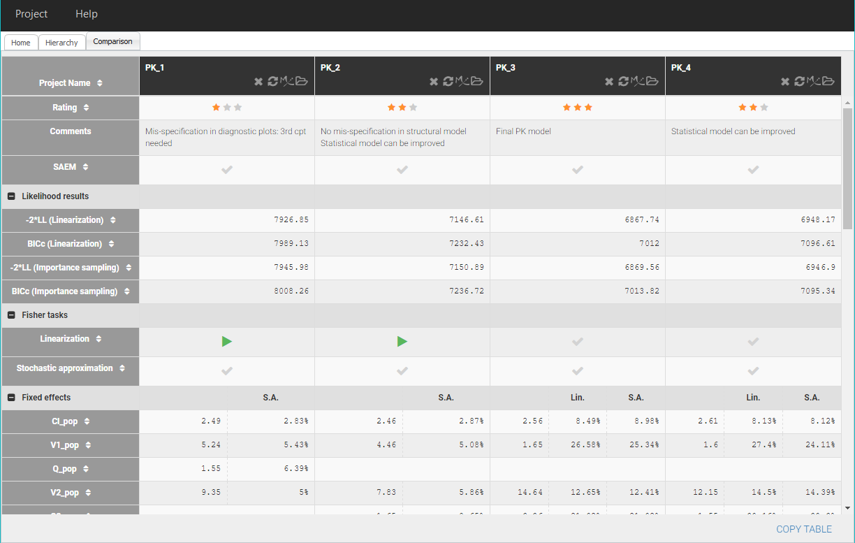
The table can be copied with the button ![]() on the bottom, to be pasted in any other software.
on the bottom, to be pasted in any other software.
Actions
Actions icons are available in the headers of the table, to perform useful actions: ![]()
Their functions are:
- Remove the project from the comparison table. This does not remove the project from the Selection panel nor theTable overview in the Hierarchy tab.
- Update the elements and results displayed for the project
- Open the project in Monolix
- Open the result folder of the project
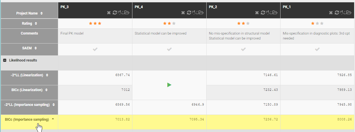
Sorting projects
Columns of the table can be reordered manually with drag-and-drop of the headers, or can be sorted in increasing or decreasing order according to the values of some row of the table, by clicking on the arrows next to the row names. Moreover, clicking on a row name colors the row in yellow to facilitate the comparison.
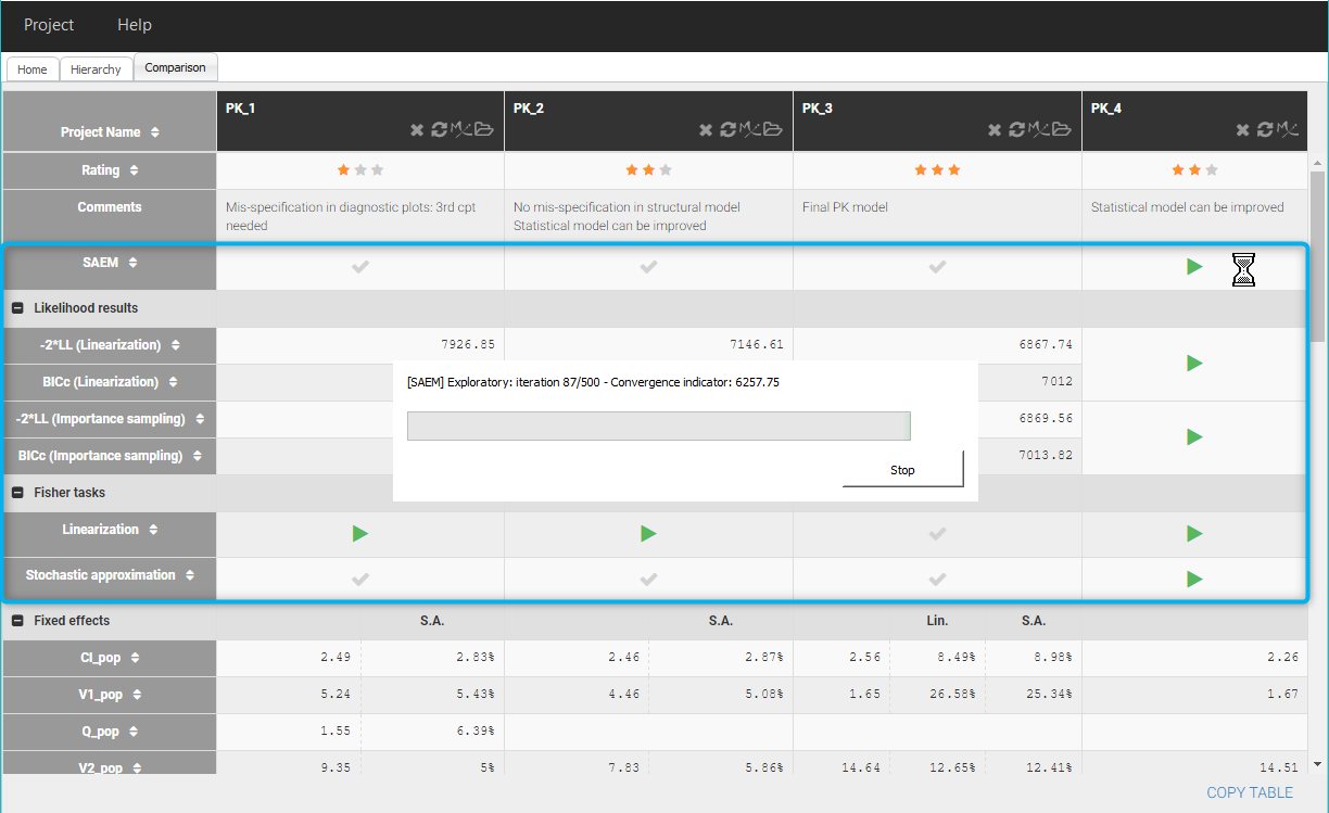
Running a task to get missing results
Some Monolix estimation tasks that have not run yet can be launched from the Comparison tab with the “Run” buttons (green arrow) to provide missing results:
- population parameters estimation with SAEM
- computing the log-likelihood by linearization or by importance sampling
- computing the standard errors with the Fisher information matrix by linearization or by sochastic approximation.
Comparing plots
For each project, diagnostic plots that have been exported as png images (this requires to generate the plots in the interface of Monolix and export them) are listed in the Figures section. Hovering on a file name colors the same diagnostic plots available for other projects, and displays a preview of the image.
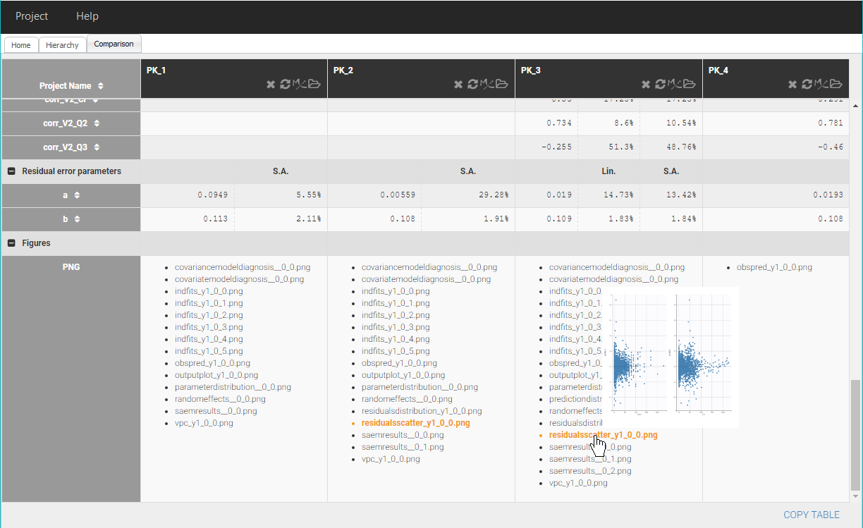
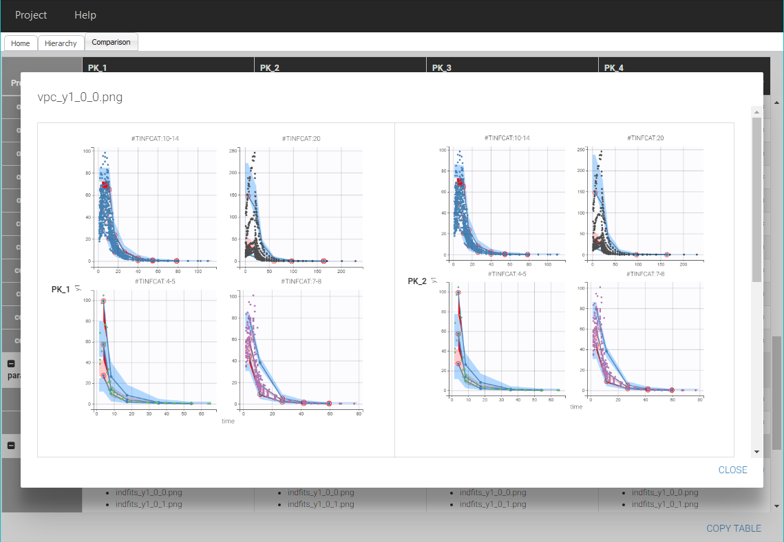
Clicking on a file name opens a window where the corresponding plot from each project of the table is displayed with the name of the project.
2.Example
In the proposed example, we use Sycomore to guide the modelling of the PKPD of remifentanil in Monolix, by providing and overview of the modelling workflow, and allowing to easily add a new step of the workflow by cloning a project to modify it.
We choose to perform a quick modelling workflow with the help of automatic model building tools, to find a good model in only a few steps:
- Insights from data exploration
- First PK model with two compartments
- Second PK model with three compartments
- Comparing two PK projects in Sycomore
- Adjusting the statistical model with Proposal
- Joint PK-PD models
- Conclusion
All modelling decisions are only summarized. You can check the detailed case study on remifentanil to read a more precise step-by-step modelling workflow with detailed explanations of each decision based on statistical tests and diagnostic plots.
Insights from data exploration
A detailed presentation and exploration of the remifentanil PKPD dataset that we wish to model is available here.
In summary, it contains:
- administration information for IV infusion,
- PK measurements of remifentanil: these observations are named y1 in Datxplore and Monolix,
- EEG measurements as PD: these observations are named y2 in Datxplore and Monolix,
- continuous covariates (age and lean body mass (LBM)), as well as categorical covariates (sex and tinfcat which is a dose group).
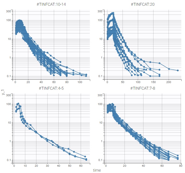
Data exploration with Datxplore or the data viewer in Monolix gives relevant insights to guide the modelling, mainly:
- The elimination shows different phases, as can be seen on the left figure below, where the PK measurements over times have been split by dose group. This means that several compartments will be needed in the PK model to capture them.
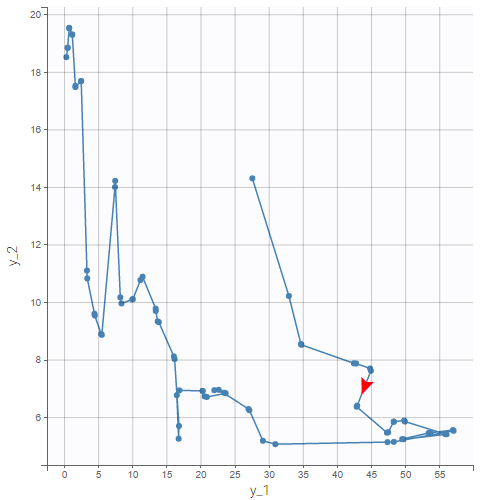
- The PD is inhibited by the PK with a delay, visible for example on the right figure below, which shows the PD over PK for id 15.
 |
 |
First PK model
Since the data exploration in Datxplore shows that a model with several compartments seems necessary to describe this dataset, we start by setting up a first PK model with two compartments in Monolix, with the following steps:
-Load the data file PKPD_data_remifentanil.csv, tag the columns as follows: ID as ID, TIME as TIME, AMT as AMOUNT, RATE as INFUSION RATE, DV as OBSERVATION, YTYPE as OBSERVATION ID, MDV as IGNORED OBSERVATION, AGE as CONTINUOUS COVARIATE, SEX as CATEGORICAL COVARIATE, LBM as CONTINUOUS COVARIATE, TINFCAT as CATEGORICAL covariate.
-Load the structural model infusion_2cpt_ClV1QV2.txt from the PK library. This is a 2 compartments model with infusion administration and linear elimination.
-Choose automatically good initial estimates for the population parameters with the “Auto-init” button in the tab “Initial estimates”.
-Keep the default statistical model.
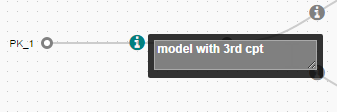
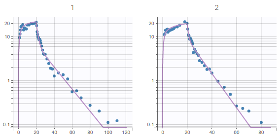
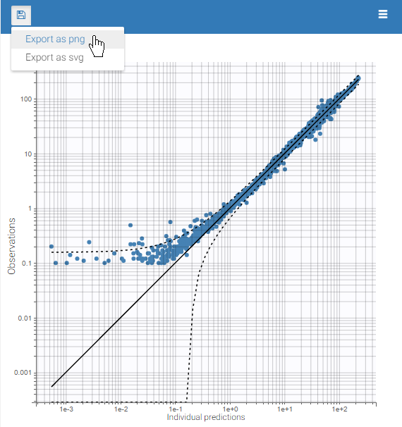
We save this first project as PK_1.mlxtran in a folder “PK”. Then, all estimation and diagnosis tasks are run to evaluate the model. In particular, the plots “Individual fits” and “Observations vs predictions” displayed below show a mis-specification of the structural model: a third compartment is needed in order to avoid under-predictions of the end of the elimination phase.
Since these plots are important to diagnose the model, we export these plots in the result folder with the button “Export as png”.
 |
 |
Finally, we note in the tab Comments the conclusion for this project: “Mis-specification in diagnostic plots: 3rd cpt needed”.
Second PK model
Next, we change the structural model to add a third compartment to the PK model. This is done by loading the structural model infusion_2cpt_ClV1Q2V2Q3V2.txt. Good initial estimates are again chosen with the button “Auto-init”.
We then save the modified project as PK_2.mlxtran in the PK folder, before running all estimation and diagnosis tasks.
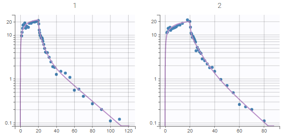
The plots “Individual fits” and “Observations vs predictions” displayed below no longer show any mis-specification of the structural model.
 |
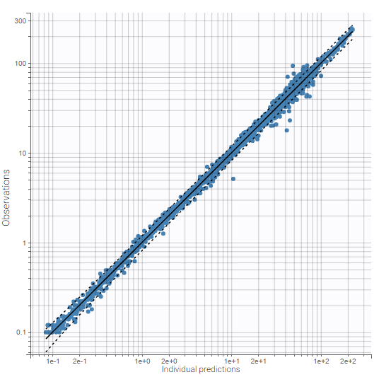 |
These plots are also exported in the Results folder. Moreover, we note in Comments: “No mis-specification in structural model”.
We can also check in the plots for individual parameters that the distributions of the individual parameters are not mis-specified.
Comparing two PK projects in Sycomore
To compare further these two projects, we create a new overview with Sycomore: after opening Sycomore and clicking on “New project”, we select the PK folder containing the two Monolix projects.
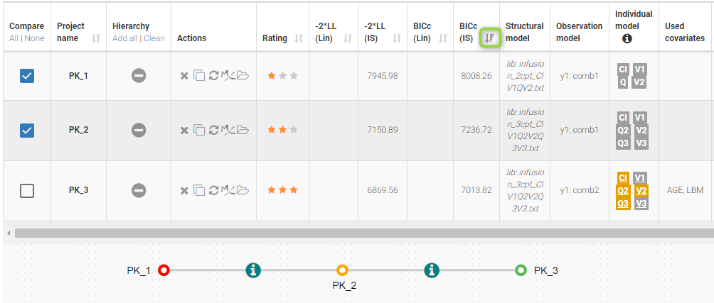
The two projects with their common folder then appear in the Selection panel on the left of the Hierarchy tab in Sycomore. After selecting them both, they also appear with their characteristics in the overview table on the top:
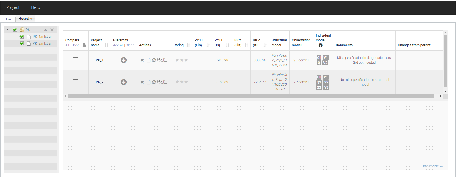
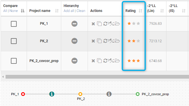
Since both projects contain the BICc computed by importance sampling, we can already see in the table that the second project PK_2 has a lower value for BICc (IS), which confirms that the fit is better. A rating can be added for each project. Here we note a rating * for PK_1 and a rating ** for PK_2.
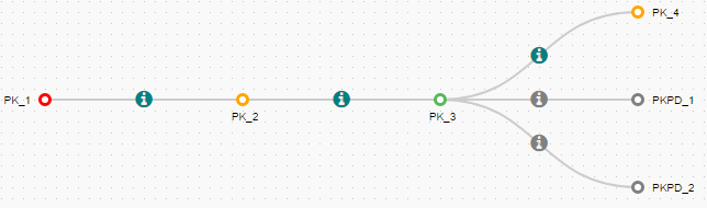
To keep track of the workflow, add these two projects in the tree view by clicking on the + icons in the column “Hierarchy”. The rating appears as a color code, with PK_1 in red and PK_2 in orange. We then drag the node PK_2 close to PK_1 to create a parent-child relationship.
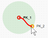
It is now possible to comment the parent-child relationship to record the changes from the parent. We write “added 3rd cpt” in the corresponding cell in the table.
We have now recorded all elements of the current workflow, thus we save the Sycomore overview as a file PKPD_remifentanil.syc. The project now looks like this:
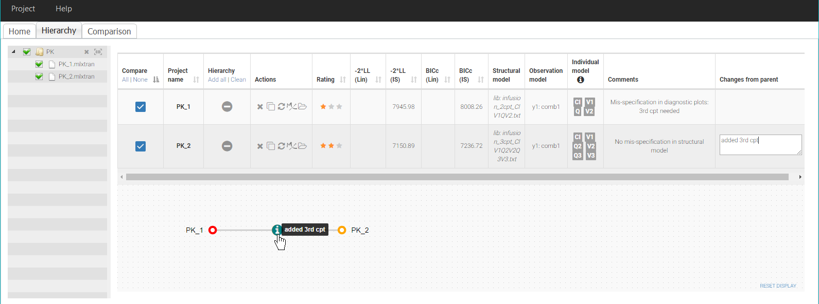
Comparing PK_1 and PK_2 in more details is also possible by selecting them both in the column Compare. The tab Comparison is then generated and allows a side-by-side comparison of the results of the projects.
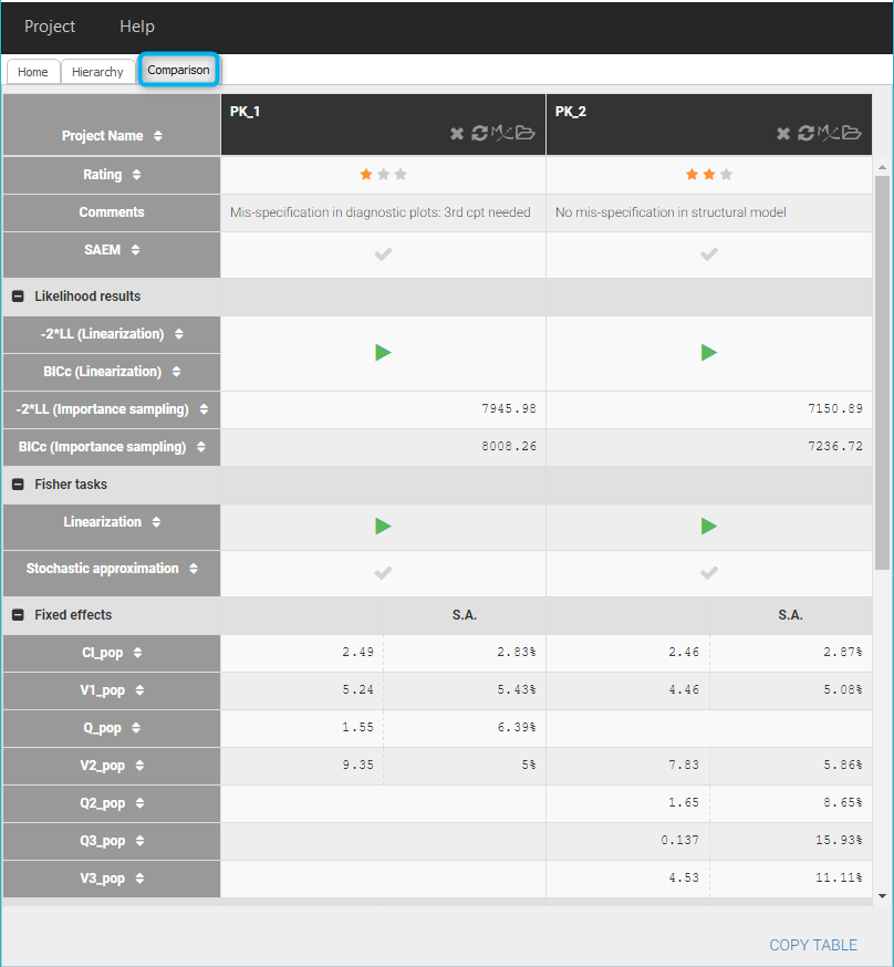
The estimates for Cl, V1 and V2 are quite close between the two projects.
The columns can be sorted according to the values of each row, and missing tasks can also be launched from there with the “run” buttons, for example if the log-likelihood has not been yet computed.
The exported plots in the section Figures can also be compared, for example as below by clicking on obspred_y1_0_0.png, which is the file name for the plot “Observation vs predictions”: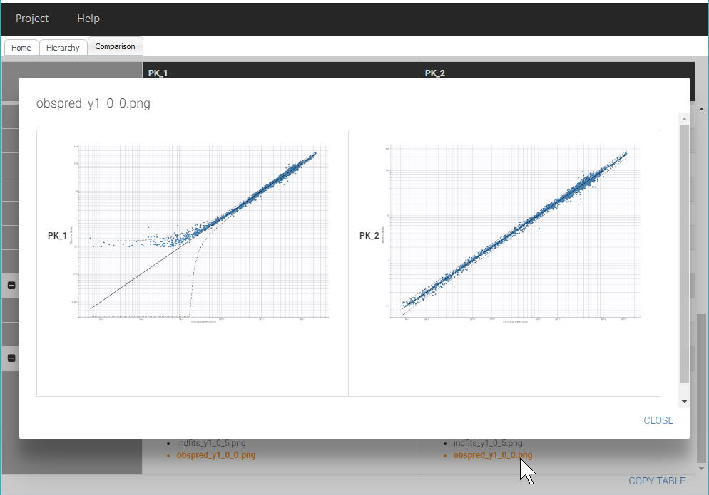
Note that we only mention a few diagnostic plots in this short case study to keep a simple workflow, however it is important to check all diagnostic plots to get a complete model diagnostic.
Adjusting the statistical model with Proposal
The structural model in PK_2 has been validated by the diagnostic plots and parameter estimation. We can now try to improve the statistical model with a different error model, covariate effects or correlations between random effects.
In a complete and detailed modelling workflow, it would be important to look at the diagnostic plots for correlations between covariates and individual parameters as well as between pairs of random effects, to detect possible effects of outliers or to identify relevant transformations for covariates before adding covariate effects. This step is neglected in this simple workflow.
For a quick improvement of the statistical model, we can look at the proposal section in the tab Results of PK_2, seen below. The aim of the Proposal is to estimate the best statistical model for the dataset, taking into account the residual error model, covariate effects and correlations between random effects.
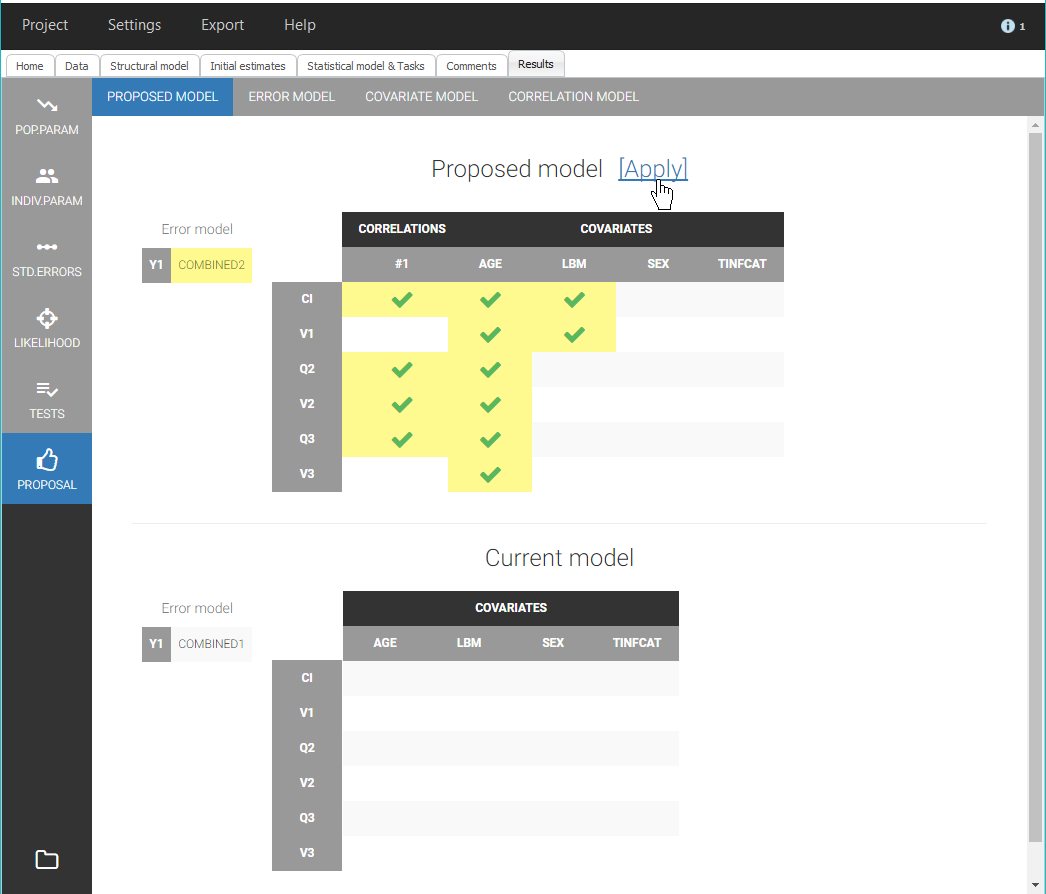
A model different than the current model is available in the tab Proposal. This proposed model includes a combined2 residual error model, covariate effects of Age on all parameters and LBM on Cl and V1, and a correlation group with the random effects of Cl, Q2, V2 and Q3. It is estimated that this model will be more performant than the current model, thus it is an interesting information that we can add in the Comments for PK_2.mlxtran with: “Statistical model can be improved”. We save PK_2.mlxtran to update its comments, and we can also update the Comments visible in Sycomore by clicking on the “refresh” button for PK_2 in the column Actions:

However the performance of the proposed model should be verified by applying the model and estimating its parameters.
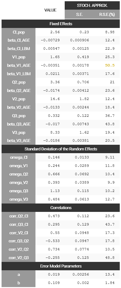
To do this, we choose the proposed model in Monolix by clicking on “Apply”, and save the modified project as PK_3.mlxtran. We run the scenario of tasks for this project, and check that the convergence of the estimates is good and that all parameters are estimated with a good confidence:
Next, we add PK_3 in the workflow overview to compare it to the previous projects, by clicking on the icon “Rescan directory” next to the PK folder in the Selection panel, like this:
This adds the project PK_3.mlxtran in the list of selected projects of the overview. It can now be added in the tree view as a child of PK_2, with the comment “Applied best proposal”.
As we can see on the table below, the BICc indeed indicates that PK_3 is more performant than PK_2, thus we choose the rating *** for PK_3. Note that BICc values can be easily compared in this table by sorting the column BICc with the button marked on the figure.
In the tab Results of Monolix for PK_3, we see that PK_3 also has a proposed model available, where a covariate effect of Sex is also included on V3, therefore, we finalize PK_3 with a comment “Proposed model available” and save.
If the proposal at the previous step has been efficient, we should not expect a large improvement of the objective function value with this new covariate effect. To check this, we apply again the best proposed model and save the modifications in a project PK_4.mlxtran. As before, it is important to not only run the scenario, but also check the convergence of the estimates and their standard errors.
Once this is done, we add PK_4 to the overview in Sycomore. Since the table is still sorted by BICc, it is quickly visible that PK_4 actually has a higher BICc than PK_3. Therefore, we choose a rating ** for PK_4 and we consider PK_3 as more performant.
We can now consider PK_3 as the final PK model. To save this decision in the comments of the project, it is possible to open again the project in Monolix directly from Sycomore, by clicking on the “Monolix” icon in the row for PK_3:
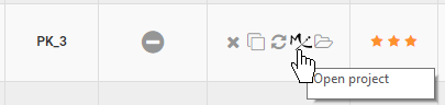
After completing the comments and saving the project, the comments displayed in Sycomore can be updated with the “refresh” button.
Joint PK-PD model
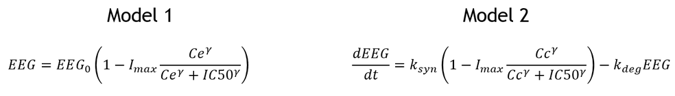
We next would like to develop a joint model for the PK and the PD. We choose to try two different PD models that could take into account the delay between remifentanil concentration and decrease of EEG, revealed by the data exporation:
- Model 1: a direct inhibition model with an effect compartment.
- Model 2: a turnover model with PD production inhibition by the PK.
Here are the equations for EEG (PD observations) for both models:
We will now define two projects with these two models, available in the libraries of Monolix, and we will then run the two projects in a row from Sycomore.
Since both PKPD models will be based on the final PK model, we start by creating two clones of PK_3 in Sycomore with the button “Clone project” (note that the action “Clone project” is also available by clicking on the node for PK_3 in the tree view):
We save each cloned project in a new folder named PKPD, under the names PKPD_1.mlxtran and PKPD_2.mlxtran. The cloned project are automatically included in the panel selection and the tree view as children nodes of PK_3:
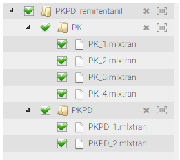 |
 |
Let’s now open PKPD_1.mlxtran in Monolix to add the first PD model.
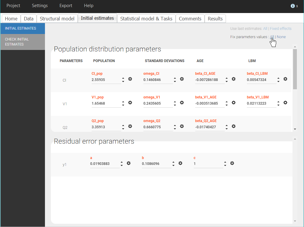
The project has been saved with the comments of PK_3, that we can delete, and the results of PK_3, which means that the PK parameters estimated with PK_3 are available. We start by defining these estimated parameters as new initial values, by clicking on “Use last estimates: all” in the tab “Initial estimates”. Then, we choose to fix all the PK population parameters: the goal is to perform a quick estimation of only the PD population parameters that will be added later in the model. To fix all population parameters, we click on “Fix parameters values: All” in the tab “Initial estimates”:
Note that this method is easy to implement in the interface of Monolix and allows to estimate only the PD population parameters, however all individual parameters will be estimated, including the PK parameters. Therefore, it will take longer than a fully sequential approach where individual PK parameters from the PK analysis are included in the dataset to be used for predictions.
We can now complete the structural model with a PD model. In the tab “Structural model”, we load a model from the PKPD models library, corresponding to the same PK model as before, with a partial inhibition PD model with effect compartment and with sigmoidicity.
We choose good initial values for the PD parameters in the panel “Check initial estimates” of the tab “Initial estimates”. The auto-init is only available for models from the PK library, therefore we have to choose manually some values that give a reasonnable fit to the data, for example ke0_pop=1, gamma_pop=2, E0_pop=20, Imax_pop=0.9, IC50_pop=10. We can then save the modified project. Since the project will be run from Sycomore, we make sure that all the tasks of the scenario are selected and saved.
We follow the same steps as for PKPD_1.mlxtran to define the second PD model in PKPD_2.mlxtran. Here we choose a PKPD model where the PD model is a turnover model with partial inhibition of the production and with sigmoidicity. We can take for initial values kout_pop=1, gamma_pop=2, R0_pop=20, Imax_pop=0.9, IC50_pop=10.
Once both projects have been defined and refreshed in Sycomore, we can launch their scenarios directly from Sycomore, by clicking in the table on the two names PKPD_1 and PKPD_2. The projects are then colored in green. The list of selected projects can then be run in a row with the button “Run”. A pop-up window opens to display the progess of the runs:
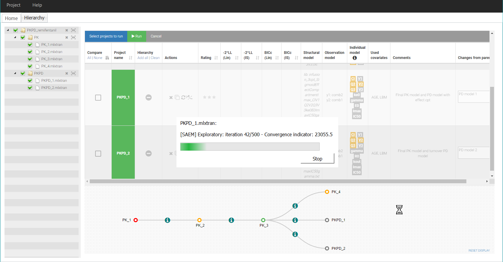
After the two runs have finished, we finally select the two PKPD projects for side-by side comparison, to check their results, in particular the estimated values and standard errors. In both cases, the parameters have been estimated with a good confidence.
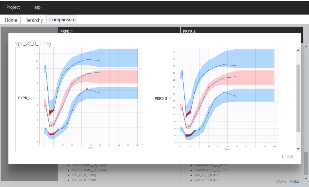
To compare the diagnostic plots, it is necessary to open the projects in the interface of Monolix to generate the plots and export them as png images. The comparison of the VPC for example shows that both models have a good predictive power:
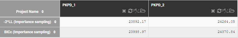
Finally, the comparison of the BICc values indicate that the model 1 is slightly more performant than model 2.
To visualize this difference on the tree view, we choose a rating *** for PKPD_1 and ** for PKPD_2.
Conclusion
We built a quick joint PKPD model for remifentanil in Monolix, with the help of structural model libraries and automatic statistical model building tools implemented in Monolix.
This example illustrates how Sycomore can be used to:
- track the steps of the modelling workflow and see at a glance the main elements of each step,
- easily add a new step of the workflow by cloning a Monolix project,
- save the changes between successive runs,
- compare side-by-side the results of similar models,
- run sets of Monolix projects.
All the material of this case study (data, Monolix projects and Sycomore overview) can be downloaded here.
3.Share your feedback
Help us improve Sycomore!
We value your opinion. We would love to hear from you to align our vision and concepts with your needs and expectations. Let’s make sure you get the most of our software.
NB: This is not a support form. Commercial users can contact us via the support email.
4.FAQ
Parameters / Prediction
- If I move the error models parameters in the interface, nothing changes. Why? This is normal. Mlxplore does not manage error models as Mlxplore focuses on predictions. Thus, if an error model is defined, the slider for the parameter can appear but will have no impact on the prediction results.
Graphics / Axis
- When I check the log y axes, an error window pops us and the axis labels of the figure are not displayed correctly. I get all zeros instead of 10^-1, 10^-2 etc. What’s going on? Read the answer here.
Graphics / IIV
- When I activate the iiv, the graphics do not display all times. Why? When the iiv is activated, draws for the covariates and/or the individual parameters are done. This can load to NaN values in the simulations for some time points. Check the warnings in the status windows. To avoid the problem, you can add saturations for example before power calculation, logarithm calculation, …
- When I check the covariate/random effect tickbox in the iiv, nothing happens. Why? When the iiv is activated (for either the individual parameters and/or the covariates), samples from the associated distribution are used. If no distribution is defined, all simulations are done with the same (population) parameters, and lead to the same prediction. This is for instance the case for covariates iiv when you export a project from Monolix. For simulation purpose in Mlxplore, the exported project takes the mean value of the covariate of the data set and set this value for Mlxplore (unique value without a distribution). You can edit your model file via the editor to add a distribution for the covariates.
Project loading
- I get an error “Load file … error” while loading a project. What can I do? If in the “Errors” tab of Mlxplore, the error is “Parse not ended”, check if your dataset file contains only allowed characters.
- I get an error “Cannot load project : parse errors” while opening Mlxplore form Monolix. What can I do? The error may be due to unallowed characters in your dataset file. Check allowed characters here.
Running a project
- I get an error “Running model error !” while running a loaded project. If in the “Errors” tab of Mlxplore, the error is “Parse not ended”, check if your dataset file contains only allowed characters.